Hidden Attractors Fractional Order: an auditable library for Chua workflows

This page introduces hidden-attractors-fo, a Python research library organized to reproduce, audit, and extend numerical experiments involving hidden-attractor candidates in integer- and fractional-order Chua/Lur’e systems.

The origin of each method remains visible in the code and documentation: Leonov—Kuznetsov for the hidden versus self-excited distinction, Danca for the non-smooth fractional Chua example, Matignon for fractional local stability, Benettin for Lyapunov exponents, Caputo for the causal fractional derivative, and Guan—Xie for the recent review of localization methods.

What The Library Does

The library separates the work into auditable tasks:

• define Chua systems and manually supplied Lur’e decompositions;
• generate describing-function/Nyquist seeds and continue them numerically;
• load real trajectories produced by workflows;
• plot phase spaces, projections, time series, spectra, and bifurcation views;
• record which diagnostics provide numerical evidence and which do not prove hiddenness.

The trajectory contract used by the examples is simple:

t,x,y,z

A project trajectory can then be loaded and plotted directly:

from hidden_attractors.io import load_trajectory_csv
from hidden_attractors.plotting import plot_phase_space

trajectory = load_trajectory_csv("outputs/.../reference_attractor.csv")
plot_phase_space(trajectory, "outputs/my_case/phase_space_3d.png")

The Integer Chua q=1 Baseline

Before extending the workflow to fractional memory, the non-smooth Chua system was verified as an order-one reference case. The stored model uses:

Parameter	Value
alpha	8.4562
beta	12.0732
gamma	0.0052
m0	-0.1768
m1	-1.1468
dynamic order	q=1.0

Its Lur’e/Nyquist describing-function closure selects omega0 = 2.03918694, k = 0.20986735, and a0 = 5.85614509, with an absolute complex closure residual of 9.93e-16.

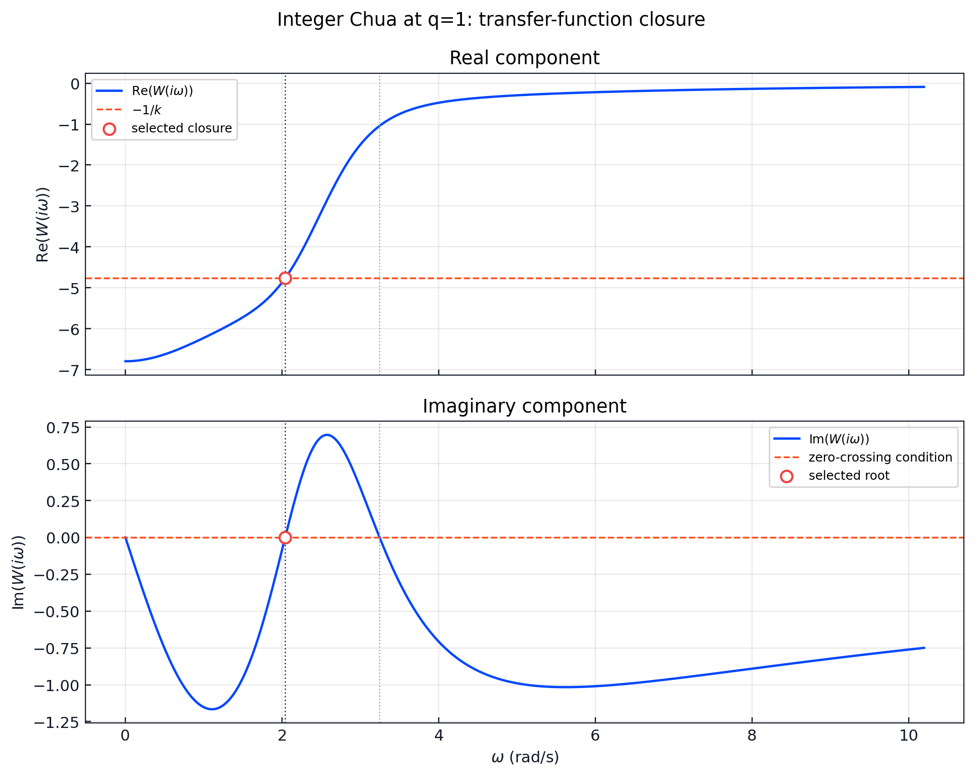
The Python workflow now generates this two-panel transfer-function check, matching the representation in the supplied MATLAB verification script: Re(W(i omega0))=-1/k and Im(W(i omega0))=0.

Published Numerical Comparison

Guan and Xie (2025), Example 6 on PDF page 14, publish the same parameter set and display the seed quantities below. The relative differences use the rounded values printed in the paper:

Quantity	Python result	Guan—Xie displayed value	Relative difference
omega0	2.039186939959001	2.0392	0.000640%
k	0.209867354515084	0.2098	0.032104%
a0	5.856145086257356	5.8576	0.024838%
y(0)	0.369331578246782	0.3694	0.018522%
z(0)	-8.366536168331880	-8.3686	0.024662%

These percentages include publication rounding and are not errors against unrounded reference data.

The harmonic seed is carried to the original nonlinear system by epsilon continuation. The regenerated run evaluates the EFORK-3 numerical route at q=1, keeping the order-one baseline directly comparable with the fractional workflow and its native validation stages.

The EFORK-3 stage order was checked against Ghoreishi, Ghaffari, and Saad (2023) and the validation implementation supplied by Dr. Luis Gerardo de la Fraga of CINVESTAV Unidad Zacatenco. The earlier integration-dependent outputs were deleted and the integer run was regenerated with K3 = a31*K1 + a32*K2.

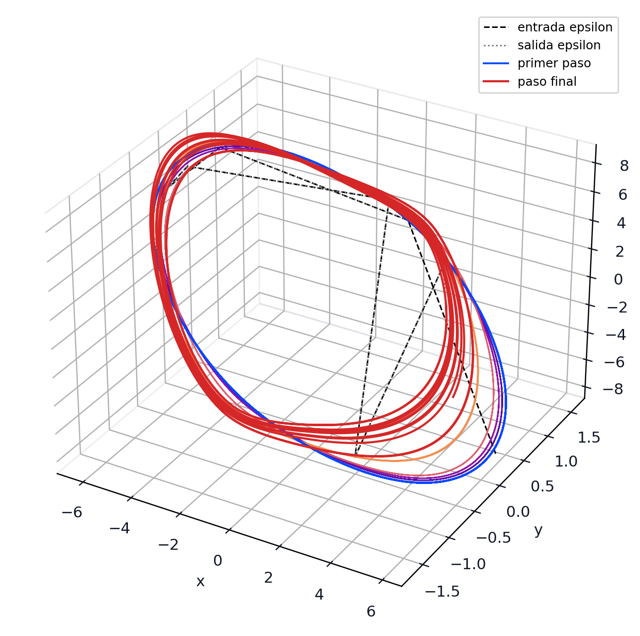
The stored final trajectory also records frequency comparisons against the describing-function seed:

Estimate	Frequency (rad/s)	Difference from omega0
Nyquist/DF seed	2.039186939959001	-
FFT of x(t)	2.303578659448180	12.9655%
Welch PSD of x(t)	2.300971181828511	12.8377%

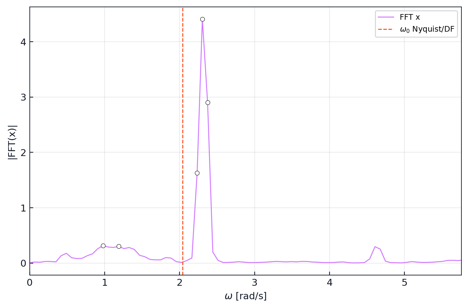
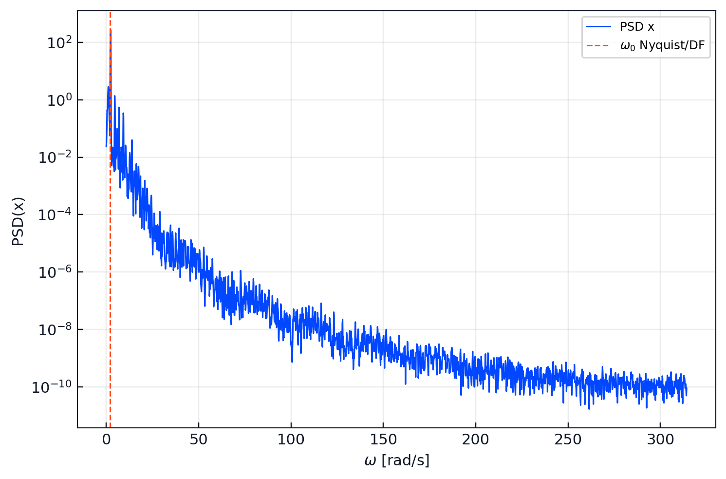
FFT and PSD are spectral diagnostics for the continued trajectory, not a hiddenness proof.

The regenerated final candidate has native Benettin Lyapunov estimates (0.20824618, 0.01373270, -1.36693009), including a positive leading exponent. Hiddenness controls launched 504 trajectories from neighborhoods of the three equilibria and recorded TARGET=0.

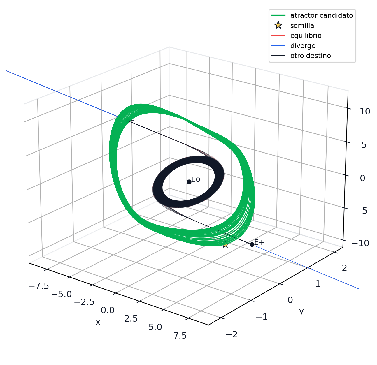
This evidence supports the wording numerical hidden-attractor candidate under the recorded finite sampling and integration horizons. It is not a global proof of hiddenness.

Fractional Non-Smooth Chua: Algebra Stage

The Danca non-smooth case at q=0.9998 is now separated from the integer baseline as its own validation target. With alpha=8.4562, beta=12.0732, gamma=0.0052, m0=-0.1768, and m1=-1.1468, MATLAB and Python reproduce the three equilibria and their regional Matignon classification: the origin is stable and the two external equilibria are unstable.

The two centered harmonic branches are:

Branch	omega0	k	a0
1	2.040286051079	0.210022792962	5.851767785486
2	3.244926730975	0.956945404928	1.053016610257

The comparison required a documented sign normalization: the Python API stores W_code = -W_report, so its residual 1 + k W_code is the same algebraic closure as the report/MATLAB residual 1 - k W_report. The supplied Wolfram source verifies the symbolic identities after renaming its protected variable Tr.

Danca (2017) is the direct publication for this exact case. Petras (2008) provides independent support for the fractional PWL Chua model family but uses other numerical parameters. Sene (2021) concerns a related fractional Chua system without the -gamma*z damping term, so it informs reporting practice rather than serving as direct numerical confirmation.

See the complete algebra audit.

Fractional-Order Outputs

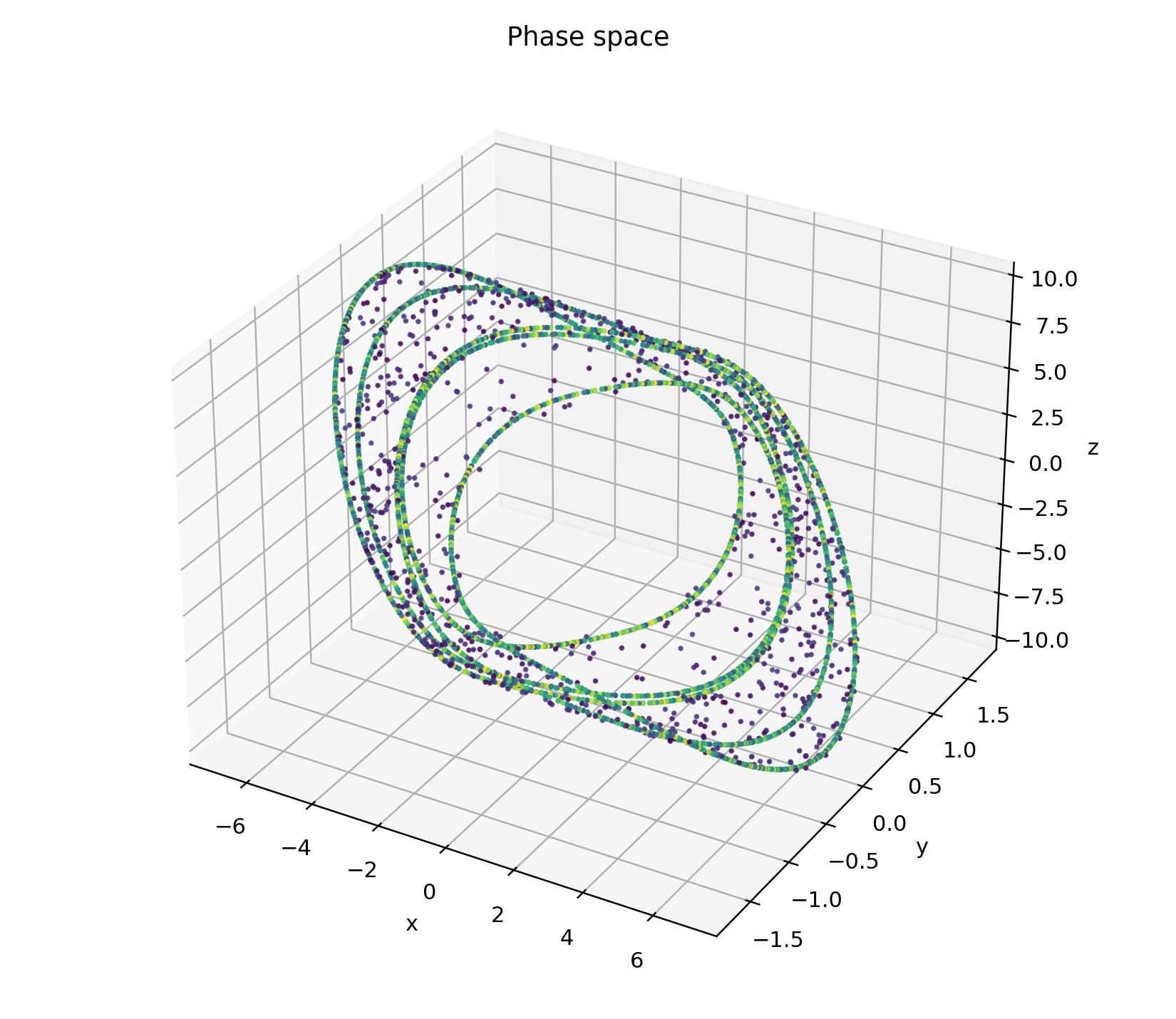
The fractional workflows retain the same evidence-first policy. The following phase portrait was generated from a real project trajectory, not from a decorative illustration.

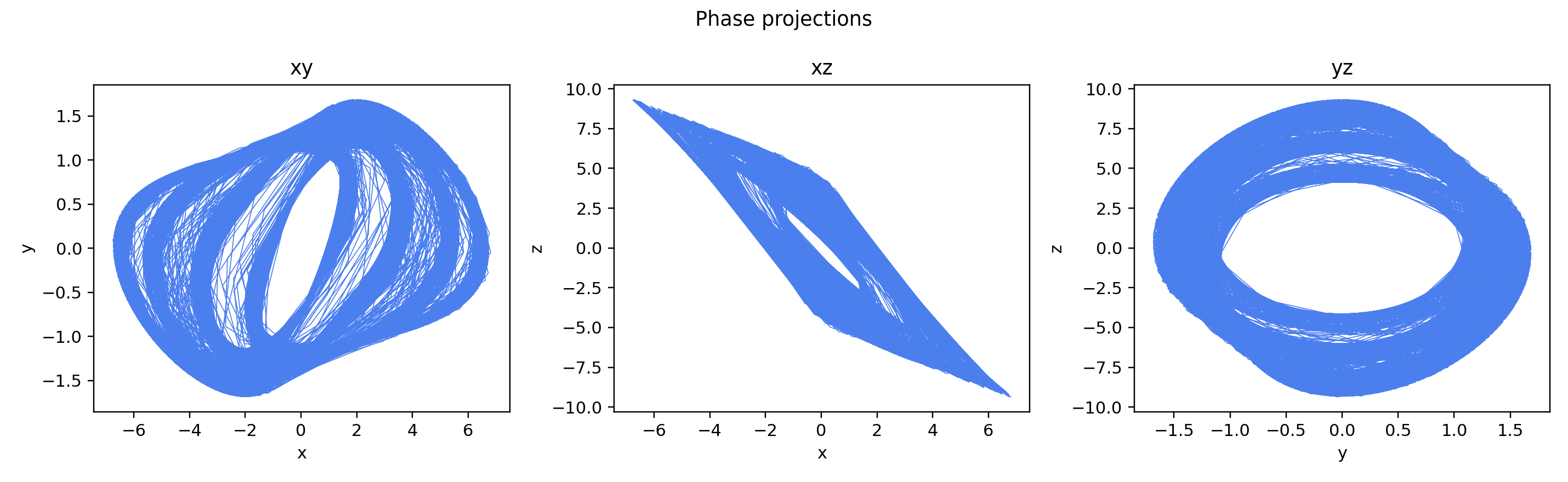
The xy, xz, and yz projections allow geometric comparisons without depending on a single three-dimensional view.

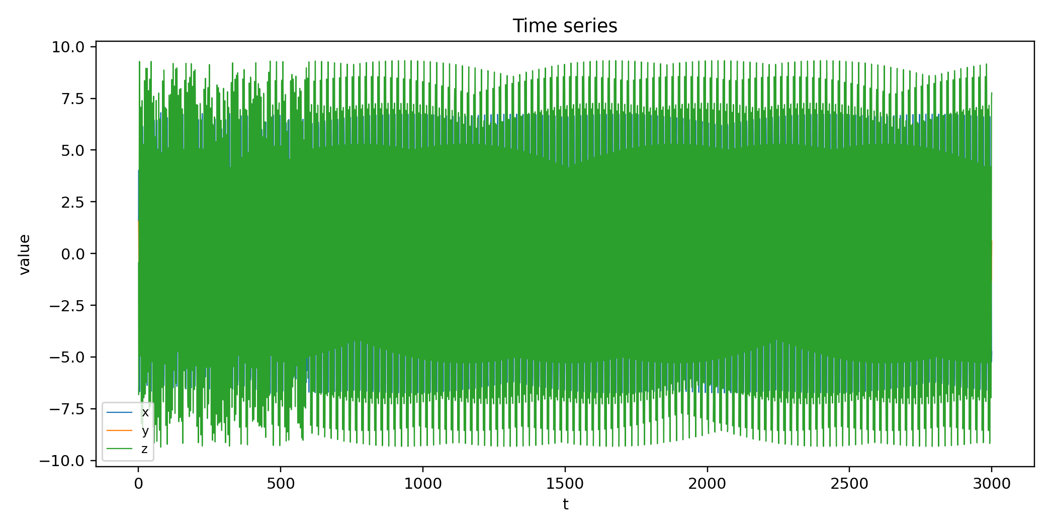
Time series help determine whether a trajectory remains bounded, collapses to an equilibrium, or requires a revised numerical contract.

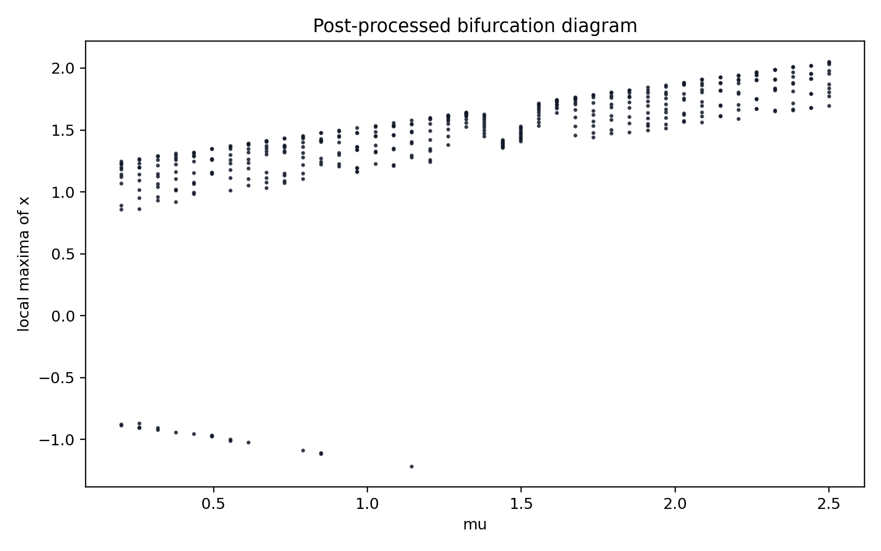
A bifurcation view extracted from previously calculated trajectories is useful post-processing evidence; it is not a substitute for full numerical continuation.

Verification Sources

The integer reference package separates each source by its evidentiary role:

Source	Current status	Role
Library artifacts in chua_integer_runs/balanced	regenerated	JSON, CSV, and figures from the corrected q=1 workflow
Theoretical report dated 17 May 2026	registered copy	Integer Chua derivation and harmonic seed; earlier integration-dependent numbers are superseded
MATLAB verifica_chua_entero.m	locally reproduced	Independent Lur’e, Nyquist/DF, canonical transform, and ODE run
Guan and Xie (2025)	published comparison	Example 6 values for omega0, k, a0, and the initial point
Wolfram Language symbolic derivation	locally executed	Algebraic verification source; intentionally performs no numerical parameter evaluation
Ghoreishi, Ghaffari, and Saad (2023) plus supplied EFORK scripts	reproduced benchmark	Tables 3, 4, 9, and 10 validate the corrected EFORK-3 stage order

Guan and Xie, A review on methods for localization of hidden attractors, published in Nonlinear Dynamics in 2025, identifies Chua’s circuit as a central historical example and reviews numerical continuation among the available localization strategies. Example 6 also supplies the rounded seed values compared above; higher-precision and spectral results come from the registered library run.

References Visible From The Code

The repository documents its calculation sources through:

• docs/references.bib;
• docs/code_reference_map.md;
• docs/integer_chua_reference.md;
• docs/reporte_unificado_chua_fraccionario.tex;
• validation/reference_cases/chua_integer_q1/.
• validation/reference_cases/efork3_ghoreishi_ghaffari/.

The rule is straightforward: a calculation must identify whether it derives from a published article, a local numerical contract, or an external reproduction tool.

Conservative Scientific Reading

A convincing trajectory is not enough to declare a hidden attractor. The documented sequence is:

harmonic seed
-> observed attractor
-> target comparison
-> numerical robustness
-> equilibrium-neighborhood probes
-> hiddenness interpretation

If a TARGET trajectory appears from an equilibrium neighborhood, the candidate must not be called hidden under that contract. This separation is what makes the library useful as scientific infrastructure rather than only a figure generator.