EFORK Solver

Extended Fractional-Order Runge-Kutta integrator: usage, memory considerations, and published validation against Ghoreishi et al. (2023).

The EFORKSolver implements an explicit Extended Fractional-Order Runge-Kutta method. It is the default solver in the hidden-attractors-fo workflows due to its excellent balance of execution speed and numerical stability.

Mathematical Preliminaries

The following definitions follow Section 2 of Ghoreishi, Ghaffari, and Saad (2023).

Riemann–Liouville Fractional Integral

Definition 1. The Riemann–Liouville fractional integral operator of order $\alpha > 0$ for a function $f(x) \in L^1[a,b]$ with $a \geq 0$ is defined as

J^{\alpha}_{a} f(x) = \frac{1}{\Gamma(\alpha)} \int_a^x (x-t)^{\alpha-1} f(t)\, dt, \qquad x \in [a,b], \quad J^0_a f(x) = f(x).

Caputo Fractional Derivative

Definition 2. The Caputo fractional derivative of order $\alpha > 0$ of a function $f(x) \in L^1[a,b]$ , with $a \geq 0$ , is defined as

{}^c_a D^\alpha_x f(x) = J^{n-\alpha}_a D^n f(x) = \begin{cases} \dfrac{1}{\Gamma(n-\alpha)} \displaystyle\int_a^x (x-t)^{n-\alpha-1} D^n f(t)\,dt, & n-1 < \alpha < n,\; n \in \mathbb{N}, \\[6pt] D^n f(x), & \alpha = n. \end{cases}

The Caputo derivative is preferred in physical modeling because its initial conditions match those of classical integer-order ODEs, giving clear physical interpretation to prescribed data.

Generalized Taylor Formula

Theorem 1 (Generalized Taylor formula for the Caputo fractional derivative). Suppose $({}^c_a D^\alpha_t)^k f(x) \in C(a,b]$ for $k = 0,1,\ldots,n+1$ , where $0 < \alpha \leq 1$ . Then, for all $x \in [a,b]$ , there exists $\xi \in (a,x)$ such that

f(x) = \sum_{i=0}^{n} \frac{(x-a)^{i\alpha}}{\Gamma(1+i\alpha)} \bigl(({}^c_a D^\alpha_t)^i f\bigr)(a) + \frac{(x-a)^{(n+1)\alpha}}{\Gamma(1+(n+1)\alpha)} \bigl(({}^c_a D^\alpha_t)^{(n+1)} f\bigr)(\xi).

Applied step-by-step from $t_n$ (not just from $t_0$ ), this formula is the foundation for deriving FORK methods that are independent of the global starting point.

Mittag-Leffler Function

Definition 3. The Mittag-Leffler function and its two-parameter form are

E_\alpha(x) = \sum_{k=0}^{\infty} \frac{x^k}{\Gamma(1+\alpha k)}, \qquad \mathfrak{R}(\alpha)>0,\; x\in\mathbb{C},

E_{\alpha,\beta}(x) = \sum_{k=0}^{\infty} \frac{x^k}{\Gamma(\beta+\alpha k)}, \qquad \mathfrak{R}(\alpha)>0,\; \beta,x\in\mathbb{C}.

Note that $E_{\alpha,1}(x) = E_\alpha(x)$ and $E_{1}(x) = e^x$ . These functions generalize the exponential and play essential roles in fractional stability analysis.

EFORK Method Definition

Consider the fractional initial-value problem with $0 < \alpha \leq 1$ :

{}^C_{t_0} D^\alpha_t\, y(t) = f(t, y(t)), \quad t \in [t_0, T], \qquad y(t_0) = y_0.

Set $t_n = t_0 + nh$ where $h = (T-t_0)/N_m$ is the step size.

Definition 4 (Ghoreishi et al. 2023, Def. 4). A family of $s$ -stage Explicit Fractional-Order Runge-Kutta (EFORK) methods is defined as

\begin{aligned} K_1 &= h^\alpha f(t_n,\, y_n),\\ K_2 &= h^\alpha f(t_n + c_2 h,\; y_n + a_{21} K_1),\\ K_3 &= h^\alpha f(t_n + c_3 h,\; y_n + a_{31} K_1 + a_{32} K_2),\\ &\;\;\vdots\\ K_s &= h^\alpha f\!\left(t_n + c_s h,\; y_n + \sum_{j=1}^{s-1} a_{sj} K_j\right), \end{aligned}

y_{n+1} = y_n + \sum_{i=1}^{s} w_i K_i,

where the unknown coefficients $\{a_{ij}\}$ and weights $\{c_i\}, \{w_i\}$ are determined by matching powers of $h^\alpha$ in the Caputo generalized Taylor expansion.

Memory Correction Term

For $n \geq 1$ , the key distinction from classical RK is the history-correction that adjusts the local Caputo derivative ${}^C_{t_n}D^\alpha_t y(t)$ to account for the trajectory before $t_n$ :

{}^C_{t_n} D^\alpha_t y(t) = F_n(t, y), \qquad F_n(t,y) = f(t,y) - \frac{1}{\Gamma(2-\alpha)} \sum_{i=0}^{n-1} \frac{y_{i+1}-y_i}{h} \left[(t-t_i)^{1-\alpha} - (t-t_{i+1})^{1-\alpha}\right].

At $n=0$ , $F_0(t,y) = f(t,y)$ (no history). For $n \geq 1$ , the sum accumulates piecewise-linear interpolation corrections from all previous steps. This convolution is the “memory” of fractional calculus and is the primary source of computational cost.

3-Stage Butcher Tableau

The three-stage EFORK method (order $3\alpha$ ) is:

\begin{array}{c|ccc} & & & \\ c_2 & a_{21} & & \\ c_3 & a_{31} & a_{32} & \\ \hline & w_1 & w_2 & w_3 \end{array}

The system of six equations (22) in Ghoreishi et al. that determine these coefficients is:

w_1+w_2+w_3 = \frac{1}{\Gamma(\alpha+1)}, \quad a_{21} = \frac{c_2^\alpha}{\Gamma(\alpha+1)}, \quad w_2 c_2^\alpha + w_3 c_3^\alpha = \frac{\Gamma(\alpha+1)}{\Gamma(2\alpha+1)},

a_{31}+a_{32} = \frac{c_3^\alpha}{\Gamma(\alpha+1)}, \quad w_2 c_2^{2\alpha}+w_3 c_3^{2\alpha} = \frac{\Gamma(2\alpha+1)}{\Gamma(3\alpha+1)}, \quad w_3\, a_{32}\, c_2^\alpha = \frac{\Gamma(\alpha+1)}{\Gamma(3\alpha+1)}.

The validated stage formula for $K_3$ used in this library is therefore:

K3 = h^alpha * F_n(t_n + c3*h,  y_n + a31*K1 + a32*K2)

where F_n includes the Caputo-history contribution at each internal stage.

Theory

The Caputo fractional derivative of order $q$ is defined as:

{}^C_0 D^q_t x(t) = \frac{1}{\Gamma(n-q)} \int_0^t \frac{x^{(n)}(\tau)}{(t-\tau)^{q-n+1}} d\tau

Because the integral evaluates the history of the function from $t=0$ , fractional derivatives possess “memory”.

The EFORK method adapts the classical 4th-order Runge-Kutta scheme to account for this memory by convolving the recent trajectory history (up to a defined memory length $N_m$ ) with a fractional weighting kernel.

Usage

from hidden_attractors.solvers import EFORKSolver
from hidden_attractors.models import rhs_nonsmooth, chua_nonsmooth_parameters

params = chua_nonsmooth_parameters()

solver = EFORKSolver(
    rhs=lambda x, t: rhs_nonsmooth(x, params),
    q=0.98,          # Fractional order (0 < q <= 1)
    dt=0.01,         # Integration time step
    memory=500       # Number of past steps to keep in memory
)

x0 = [0.1, 0.0, 0.0]
t_span = (0.0, 100.0)

t, x = solver.integrate(x0, t_span)

Batch Processing

If you pass a 2D array of initial conditions (shape (N, 3)) to solver.integrate(), the solver will integrate all trajectories simultaneously. If the C backend is active, this loop is parallelized using OpenMP.

import numpy as np

# 50 random initial conditions
X0 = np.random.rand(50, 3) 

# Integrate all 50 trajectories
t, X = solver.integrate(X0, t_span)

print(X.shape) # (10001, 50, 3) -> (time_steps, n_trajectories, dimensions)

Memory Considerations

The memory parameter dictates how many previous states are used to evaluate the next step.

A memory of 500 with dt=0.01 means the system “remembers” the last 5.0 seconds of simulation.
As memory increases, the computational cost per step increases linearly.
If the simulation time exceeds the memory window, the oldest states are discarded (sliding window approximation).

Published Validation

The three-stage EFORK implementation is validated independently from any chaotic-system classification using the manufactured-solution examples in Ghoreishi, Ghaffari, and Saad (2023).

Validated Stage Formula

The published method evaluates

K3 = h^alpha F_n(t_n + c3 h, y_n + a31 K1 + a32 K2)

where F_n includes the known Caputo-history contribution at each internal stage. This is also the ordering used by the independent ejemplo1.py script supplied by Dr. Luis Gerardo de la Fraga of CINVESTAV Unidad Zacatenco.

Published Tables Reproduced

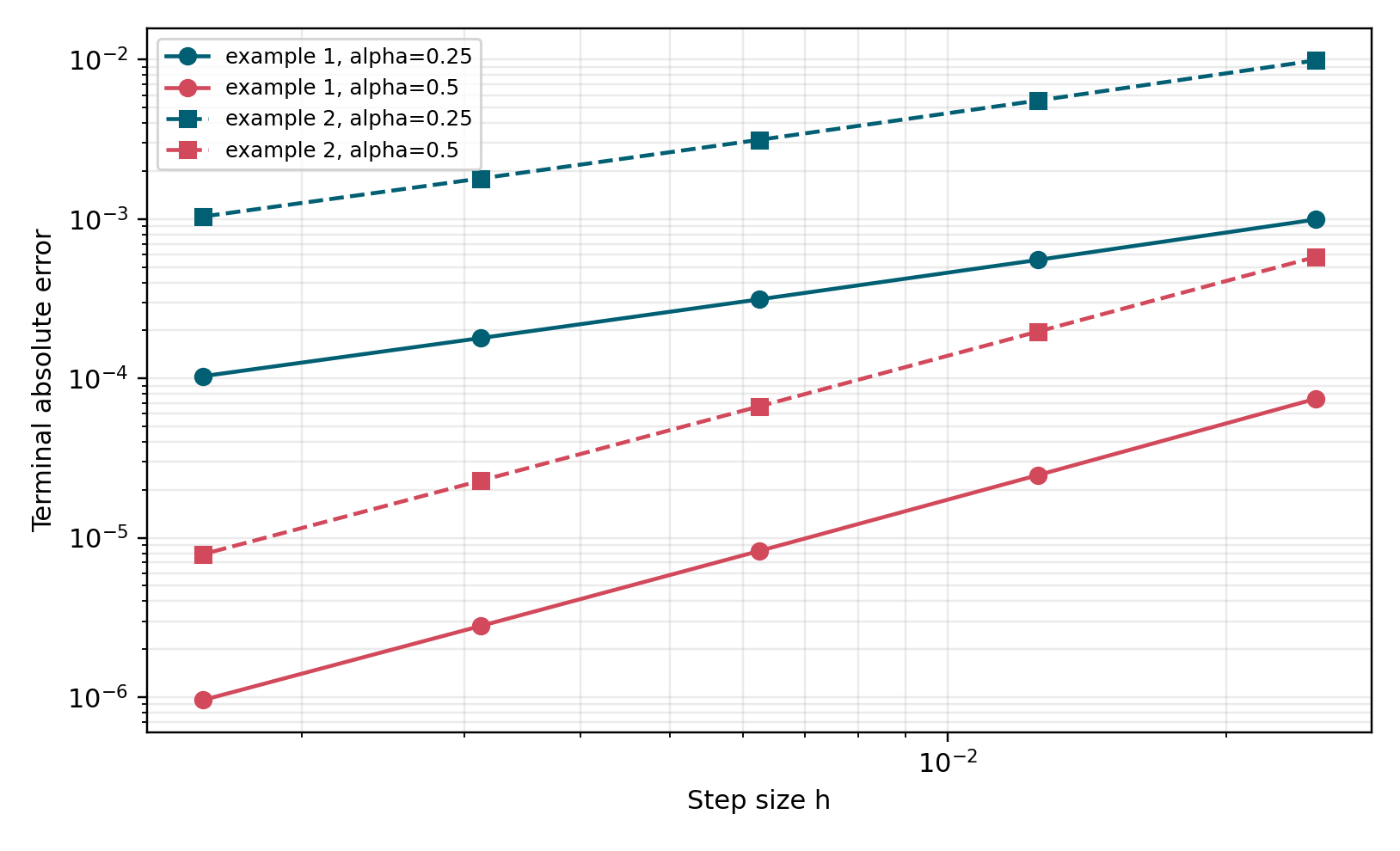
The validation runs Examples 1 and 2 at T=1, for N = 40, 80, 160, 320, 640.

Table	Example	Fractional order	Status
3	Example 1	0.25	Reproduced
4	Example 1	0.50	Reproduced
9	Example 2	0.25	Reproduced
10	Example 2	0.50	Reproduced

The largest absolute difference from a displayed paper value is 5.5489224e-9, within a 6e-9 threshold selected for the article’s printed rounding.

EFORK-3 manufactured-solution convergence

Registered Evidence

The library validation package contains the computed CSV, the machine-readable summary, the convergence plot above, and source-hashed copies of constantes_efork.py and ejemplo1.py:

version_2/validation/reference_cases/efork3_ghoreishi_ghaffari/

This numerical-method validation is separate from the integer Chua hidden-attractor reference run. A chaotic trajectory is only reported after its integration-dependent outputs have been calculated with the corrected validated stage ordering.

It validates the published EFORK-3 reference implementation and the corrected q=1 rerun; it does not by itself validate truncated-memory fractional native trajectories. Those require separate fractional evidence.

Reference

F. Ghoreishi, R. Ghaffari, and N. Saad, “Fractional Order Runge-Kutta Methods,” Fractal and Fractional, vol. 7, article 245, 2023.