Chua Integer q=1 Reference

Verified order-one Chua benchmark used to start the reusable hidden-attractor workflow.

The integer-order Chua case is the reference point for the workflow. It is evaluated at $q=1$ within the same numerical family used to extend the analysis to fractional order. This allows the Lur’e decomposition, describing function, continuation process, and hiddenness controls to be audited before fractional memory is introduced.

Verified Model

\begin{aligned} \dot{x} &= \alpha\left(y-x-f(x)\right),\\ \dot{y} &= x-y+z,\\ \dot{z} &= -(\beta y+\gamma z),\\ f(x) &= m_1x+(m_0-m_1)\operatorname{sat}(x). \end{aligned}

Parameter	Value
$\alpha$	8.4562
$\beta$	12.0732
$\gamma$	0.0052
$m_0$	-0.1768
$m_1$	-1.1468
Dynamic order	$q=1$

The registered decomposition is

\dot{X}=PX+q_v\psi(r^TX), \qquad r^TX=x,

with

P=\begin{bmatrix} 1.24137016 & 8.4562 & 0\\ 1 & -1 & 1\\ 0 & -12.0732 & -0.0052 \end{bmatrix}, \quad q_v=\begin{bmatrix}-8.4562\\0\\0\end{bmatrix}, \quad r=\begin{bmatrix}1\\0\\0\end{bmatrix}.

The recorded algebraic residual for this Lur’e representation is zero in the numerical check.

Harmonic Closure And Seed

The selected Nyquist/describing-function branch produces:

Quantity	Value
$\omega_0$	2.039186939959001
$k$	0.209867354515084
$a_0$	5.856145086257356
$	W(i\omega_0)N(a_0)+1
Seed $X_0$	$(5.85614509,\ 0.36933158,\ -8.36653617)$

Real and imaginary transfer-component closure for integer Chua

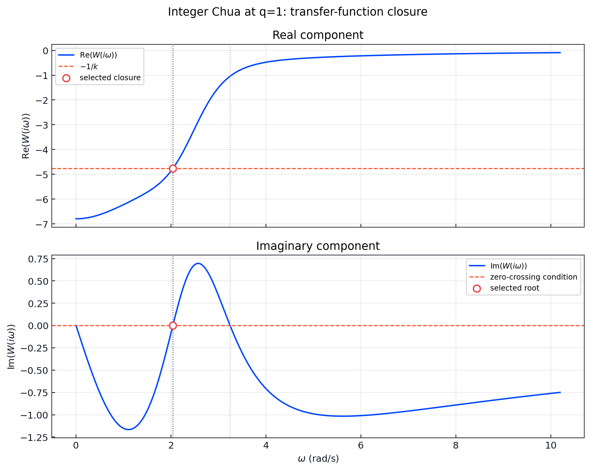
The Python workflow generates these panels to match the verification view in the supplied MATLAB script: the upper panel checks $\operatorname{Re}(W(i\omega_0))=-1/k$ , and the lower panel checks $\operatorname{Im}(W(i\omega_0))=0$ .

Comparison With The Published Example

Guan and Xie (2025), Example 6 on PDF page 14, publish this same parameter set and display $\omega_0=2.0392$ , $k=0.2098$ , $a_0=5.8576$ , and $X_0=(5.8576,\ 0.3694,\ -8.3686)$ . Comparing the Python output to those printed values gives:

Quantity	Python result	Paper value	Relative difference
$\omega_0$	2.039186939959001	2.0392	0.000640%
$k$	0.209867354515084	0.2098	0.032104%
$a_0$	5.856145086257356	5.8576	0.024838%
$y(0)$	0.369331578246782	0.3694	0.018522%
$z(0)$	-8.366536168331880	-8.3686	0.024662%

These differences include the four-decimal rounding in the published display; they are not errors against unrounded paper data.

The EFORK-3 stage ordering was subsequently checked against Ghoreishi, Ghaffari, and Saad (2023) and the validation script supplied by Dr. Luis Gerardo de la Fraga (CINVESTAV Unidad Zacatenco). The earlier integration-dependent outputs were deleted and recalculated with K3 = a31*K1 + a32*K2.

The seed is transported by continuation in $\varepsilon$ through $\varepsilon=1$ , where the recorded final state is $(1.99297400,\ 1.26397185,\ -2.55106335)$ .

Continuation from harmonic seed to the original system

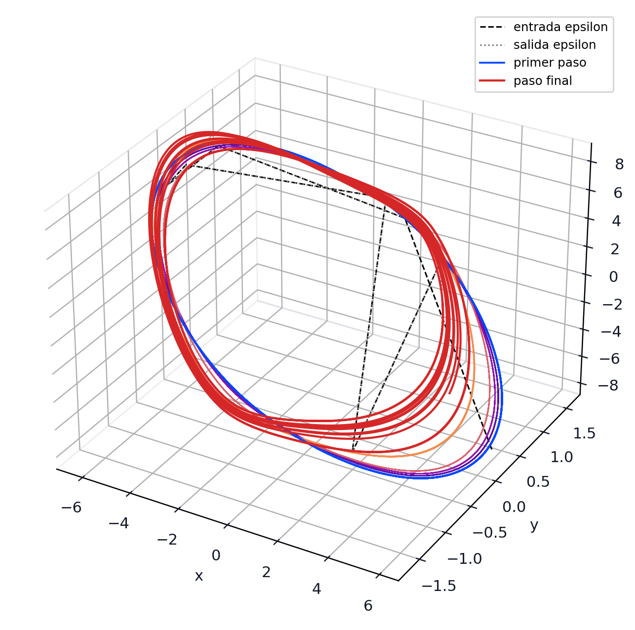
Spectral Consistency Diagnostic

The stored final x(t) trajectory provides an additional comparison with the seed frequency:

Estimate	Frequency (rad/s)	Difference from $\omega_0$
Nyquist/DF seed	2.039186939959001	-
Direct FFT of $x(t)$	2.303578659448180	12.9655%
Welch PSD of $x(t)$	2.300971181828511	12.8377%

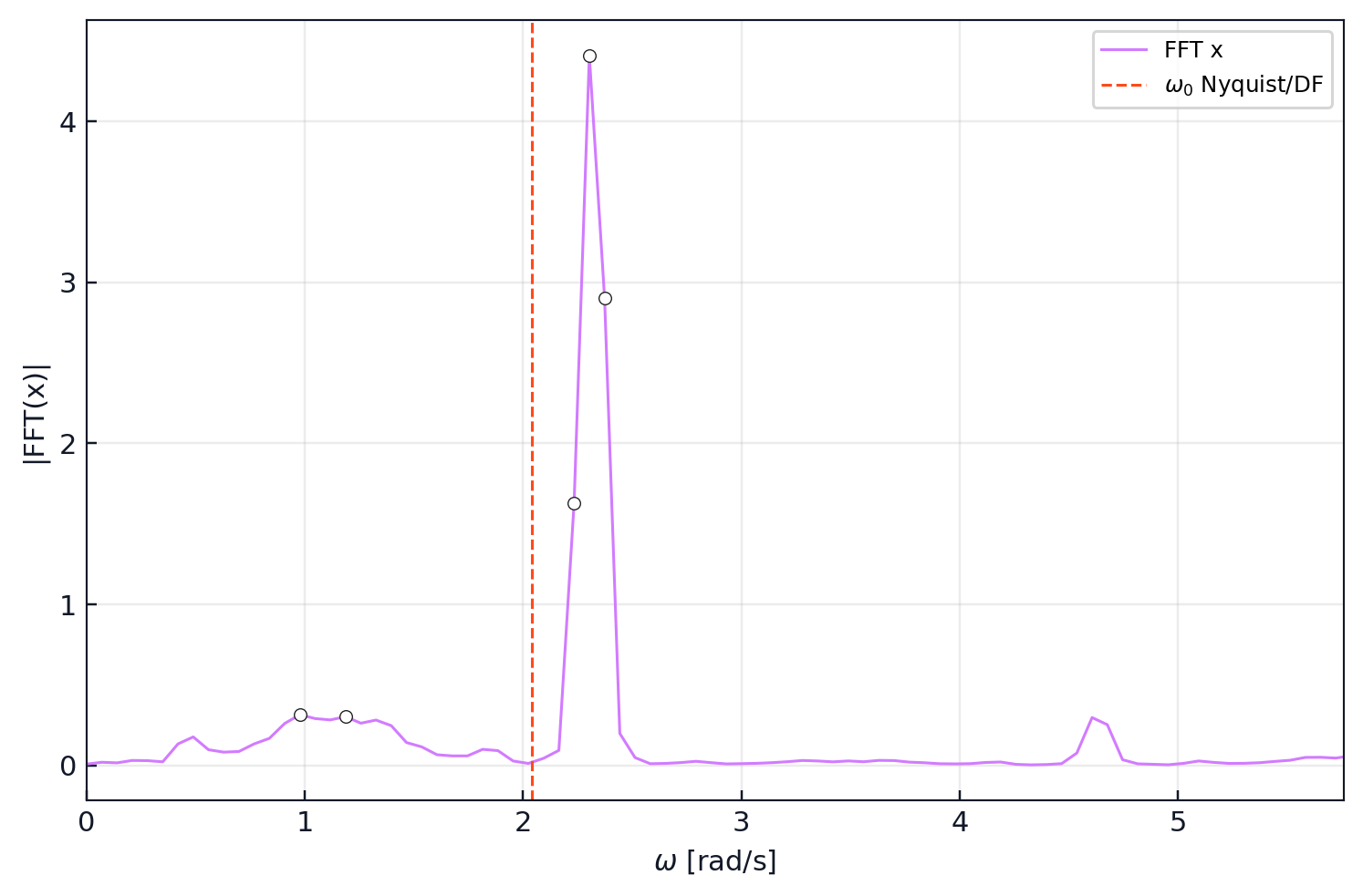
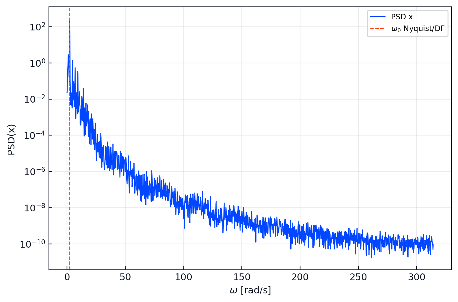
FFT frequency comparison for integer Chua

PSD frequency comparison for integer Chua

The describing function generates a first-harmonic seed; the final chaotic trajectory can have shifted dominant spectral content. FFT and PSD are diagnostics, not hiddenness proofs.

Dynamic And Hiddenness Evidence

The numerical process uses EFORK-3 evaluated at $q=1$ ; the heavy basin, hiddenness, and exponent checks run through the native workflow backends. This preserves comparability with the fractional route.

Evidence	Recorded result
Effective attractor seed	$(4.09187265,\ -0.08387100,\ -7.50907585)$
Lyapunov exponents	$(0.20824618,\ 0.01373270,\ -1.36693009)$
Controlled equilibria	$E_0$ , $E_+$ , $E_-$
Neighborhood probes	504
Trajectories reaching the target	`TARGET=0`

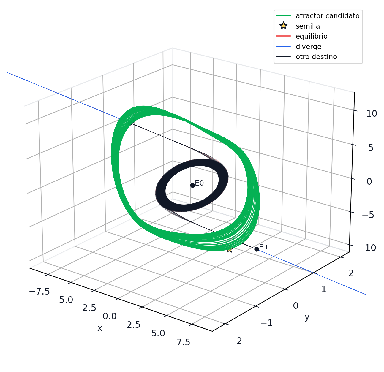
Control trajectories from equilibrium neighborhoods

The absence of TARGET hits supports the classification numerical hidden-attractor candidate under the recorded sampling and horizons. It is not presented as a global proof.

Verification Sources

Source	Incorporated scope
Theoretical report `170526.pdf` dated 17 May 2026	Lur’e derivation and harmonic seed; its earlier integration-dependent values are superseded by the corrected run.
Library artifacts in `chua_integer_runs/balanced`	Regenerated JSON, CSV, and figures recording corrected EFORK-3 at $q=1$ .
MATLAB `verifica_chua_entero.m`	Locally executed reproduction of Lur’e form, harmonic closure, canonical transform, and integer ODE comparison.
Guan and Xie (2025)	Published Example 6 values for $\omega_0$ , $k$ , $a_0$ , and the initial point used in the comparison table.
Wolfram Language `chua_entero_algebraico_sin_numericos.wl`	Locally executed symbolic derivation; by design it contains no numerical parameter evaluation.
Ghoreishi, Ghaffari, and Saad (2023) plus the supplied EFORK script	Reproduced Tables 3, 4, 9, and 10 validating the corrected stage ordering.

The promoted evidence is organized in version_2/validation/reference_cases/chua_integer_q1/, separately from the main fractional contract to avoid mixing systems and tolerances.

Bibliographic Reference

X. Guan and Y. Xie, “A review on methods for localization of hidden attractors,” Nonlinear Dynamics, vol. 113, pp. 22223-22255, 2025. DOI: 10.1007/s11071-025-11327-5.

F. Ghoreishi, R. Ghaffari, and N. Saad, “Fractional Order Runge-Kutta Methods,” Fractal and Fractional, vol. 7, article 245, 2023.